前言

Autoencoder 是一個非常重要的模型，它是很多進階模型的基礎，例如風格轉換(Style Transfer)、影像分割(Image Segmentation)、對抗生成網路(GAN)、WaveNet，所以，花一些篇幅說明此一模型。

Autoencoder 結構

Autoencoder包含兩部份：

1. 編碼器(Encoder)：就是萃取特徵的過程，類似前面CNN模型，不含最後的分類層(Dense)。
2. 解碼器(Decoder)：根據萃取的特徵重建影像。

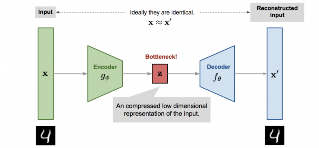
圖一. Autoencoder 結構，圖片來源：AutoEncoder (一)-認識與理解

編碼再解碼，乍聽起來好像多此一舉，關鍵在於萃取特徵，它會取得圖像的主要特徵，其他非特徵的訊號會被濾掉，所以，根據萃取的特徵重建影像，這些非特徵的訊號並不會包含在內，就可以達到去除雜訊的目的，不管圖像、聲音都可以利用此一模型的變形(Variants)去除雜訊。

實作

我們就作一個實驗，把 MNIST 的原始資料隨機加一些雜訊，然後，利用 Autoencoder 模型訓練，看看效果如何。程式分段說明如下：

1. 匯入套件、設定超參數。

import numpy as np
import tensorflow as tf
import tensorflow.keras as K
import matplotlib.pyplot as plt
from tensorflow.keras.layers import Dense, Conv2D, MaxPooling2D, UpSampling2D

# 超參數設定
batch_size = 128
max_epochs = 50
filters = [32,32,16]

2. 取得 MNIST 訓練資料

# 只取 X ，不須 Y
(x_train, _), (x_test, _) = K.datasets.mnist.load_data()

# 常態化
x_train = x_train / 255.
x_test = x_test / 255.

# 加一維：色彩
x_train = np.reshape(x_train, (len(x_train),28, 28, 1))
x_test = np.reshape(x_test, (len(x_test), 28, 28, 1))

3. 在既有圖片加雜訊

noise = 0.5
# 隨機加雜訊
x_train_noisy = x_train + noise * np.random.normal(loc=0.0, scale=1.0, size=x_train.shape)
x_test_noisy = x_test + noise * np.random.normal(loc=0.0, scale=1.0, size=x_test.shape)

# 加完裁切數值，不大於 1
x_train_noisy = np.clip(x_train_noisy, 0, 1)
x_test_noisy = np.clip(x_test_noisy, 0, 1)

x_train_noisy = x_train_noisy.astype('float32')
x_test_noisy = x_test_noisy.astype('float32')

4. Input 資料製造好了，接著建立模型，先建立編碼器(Encoder)模型，使用CNN的捲積(Conv2D)及池化(Pool)層。模型建立採 Subclass 方式，初始化函數(init)建立各種捲積層，call 函數把各層連接起來。

# 編碼器(Encoder)
class Encoder(K.layers.Layer):
    def __init__(self, filters):
        super(Encoder, self).__init__()
        self.conv1 = Conv2D(filters=filters[0], kernel_size=3, strides=1, activation='relu', padding='same')
        self.conv2 = Conv2D(filters=filters[1], kernel_size=3, strides=1, activation='relu', padding='same')
        self.conv3 = Conv2D(filters=filters[2], kernel_size=3, strides=1, activation='relu', padding='same')
        self.pool = MaxPooling2D((2, 2), padding='same')
               
    
    def call(self, input_features):
        x = self.conv1(input_features)
        #print("Ex1", x.shape)
        x = self.pool(x)
        #print("Ex2", x.shape)
        x = self.conv2(x)
        x = self.pool(x)
        x = self.conv3(x)
        x = self.pool(x)
        return x

5. 建立解碼器(Decoder)模型如下，upsample與池化層相反，把一個點變成一個面，例如 2x2 共4個點。

class Decoder(K.layers.Layer):
    def __init__(self, filters):
        super(Decoder, self).__init__()
        self.conv1 = Conv2D(filters=filters[2], kernel_size=3, strides=1, activation='relu', padding='same')
        self.conv2 = Conv2D(filters=filters[1], kernel_size=3, strides=1, activation='relu', padding='same')
        self.conv3 = Conv2D(filters=filters[0], kernel_size=3, strides=1, activation='relu', padding='valid')
        self.conv4 = Conv2D(1, 3, 1, activation='sigmoid', padding='same')
        self.upsample = UpSampling2D((2, 2))
  
    def call(self, encoded):
        x = self.conv1(encoded)
        # 上採樣
        x = self.upsample(x)

        x = self.conv2(x)
        x = self.upsample(x)
        
        x = self.conv3(x)
        x = self.upsample(x)
        
        return self.conv4(x)

6. 整合編碼器(Encoder)、解碼器(Decoder) 模型為Autoencoder 結構，解碼器接在編碼器後面。

class Autoencoder(K.Model):
    def __init__(self, filters):
        super(Autoencoder, self).__init__()
        self.loss = []
        self.encoder = Encoder(filters)
        self.decoder = Decoder(filters)

    def call(self, input_features):
        #print(input_features.shape)
        encoded = self.encoder(input_features)
        #print(encoded.shape)
        reconstructed = self.decoder(encoded)
        #print(reconstructed.shape)
        return reconstructed

7. 訓練模型。

model = Autoencoder(filters)

model.compile(loss='binary_crossentropy', optimizer='adam')

loss = model.fit(x_train_noisy,
                x_train,
                validation_data=(x_test_noisy, x_test),
                epochs=max_epochs,
                batch_size=batch_size)

8. 訓練完，繪製損失函數

plt.plot(range(max_epochs), loss.history['loss'])
plt.xlabel('Epochs')
plt.ylabel('Loss')
plt.show()

9. 比較加了雜訊的圖與訓練後的圖。

number = 10  # how many digits we will display
plt.figure(figsize=(20, 4))
for index in range(number):
    # display original
    ax = plt.subplot(2, number, index + 1)
    plt.imshow(x_test_noisy[index].reshape(28, 28), cmap='gray')
    ax.get_xaxis().set_visible(False)
    ax.get_yaxis().set_visible(False)

    # display reconstruction
    ax = plt.subplot(2, number, index + 1 + number)
    plt.imshow(tf.reshape(model(x_test_noisy)[index], (28, 28)), cmap='gray')
    ax.get_xaxis().set_visible(False)
    ax.get_yaxis().set_visible(False)
plt.show()

結果如下，上圖為加了雜訊的圖，下圖為訓練後的圖，真的做到了。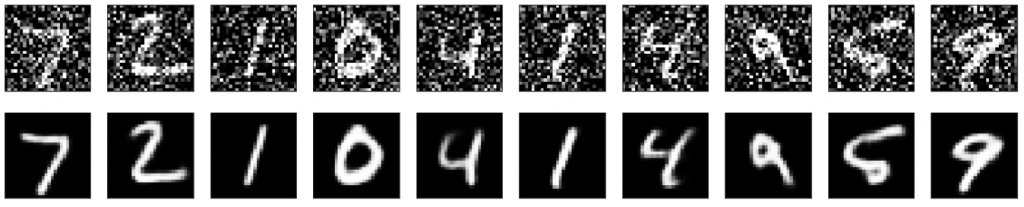

結論

Autoencoder 搞定了，我們下一篇就來看一個變形 U-Net，它被廣泛被應用醫療影像的識別。

本篇範例包括 19_01_Image_Autoencoder.ipynb，可自【這裡】下載。