今日大綱

• 資料集
• 評估指標
• 程式碼

資料集

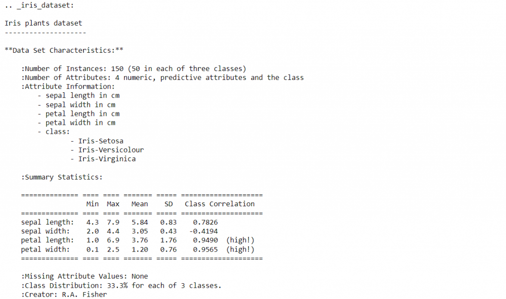
邏輯斯迴歸實作我以常見的鳶尾花(Iris)資料集當作範例，在機器學習開源資料集網站UCI，或是sklearn library都可以下載。獨立變數為花萼長度 (sepal length)、花萼寬度 (sepal width)、花瓣長度 (petal length)以及花瓣寬度 (petal width)，單位為公分，而依變數為種類，總共有三個，分別為山鳶尾 (Iris Setosa)、變色鳶尾 (Iris Versicolor)以及維吉尼亞鳶尾 (Iris Virginica)。

評估指標

1. 混淆矩陣 (Confusion matrix)
   根據實際值與預測值將樣本分為四個，第一個是True positive (TP)，也就是實際值與預測值皆為1；第二個是False negative (FN)，實際值為1，預測值為0；第三個是False positive (FP)，實際值為0，預測值為1；最後一個是True negative (TN)，實際值與預測值皆為0。

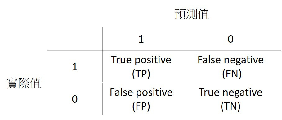
很多人很容易把False negative與False positive搞混，在記的時候我是以預測值的角度去看，False negative就是預測值為0，False positive就是預測值為1。

• 準確率 (Accuracy)
  準確率為所有樣本中，預測正確結果所佔的比例。
  準確率雖然越高越好，但並不一定適用於每個模型，如果1000筆資料中，負樣本數只有5筆，那模型將所有資料都預測為正樣本，準確率也高達99.5%。雖然這個例子較極端，但現實世界的資料大部分分布不均，正樣本或負樣本比較多。

• 精確率 (Precision)
  精確率為預測值為正的樣本中，正確預測為正樣本的結果所佔的比例。
  

• 召回率 (Recall)
  召回率為實際為正的樣本中，正確預測為正樣本的結果所佔的比例。
  

• F1值 (F1-Score)
  F1值為精確率與召回率的結合，用來衡量演算法表現好壞。
  

3. AUC (Area under curve, 曲線下面積)
   AUC為ROC (Receiver operating characteristic)下的面積，ROC曲線的橫軸為偽陽性率 (False positive rate, FPR)，縱軸為真陽性率 (True positive rate, TPR)，與召回率相同。

如果AUC等於0.5，代表模型效果與隨機預測相同，因此大部分以0.5當作判斷基準，如果高於0.5，代表模型具有預測效果；反之，分類器預測效果還比隨機預測差。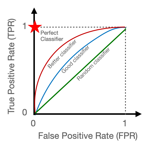

圖片來源:https://towardsdatascience.com/a-quick-guide-to-auc-roc-in-machine-learning-models-f0aedb78fbad

程式碼

首先，將鳶尾花的資料匯入，資料型態為字典，印出資料集的敘述以檢視獨立變數與目標變數。

from sklearn.datasets import load_iris
import pandas as pd
import matplotlib.pyplot as plt
data = load_iris()
print(data.DESCR)

將資料存至x與y變數中，並且取出目標函數的名稱，總共有三個不同的鳶尾花品種

x = pd.DataFrame(data['data'])
#data的feature_names指定成x的column名稱
x.columns = data['feature_names']
y = data['target']
targets = data['target_names']
print(targets)

將資料切割成訓練集與測試集，進一步訓練Logistic regression模型，並且預測測試集裡的資料。

from sklearn.model_selection import train_test_split
from sklearn.linear_model import LogisticRegression
x_train, x_test, y_train, y_test = train_test_split(x, y, test_size = 0.2, random_state = 1)
classifier = LogisticRegression()
classifier.fit(x_train, y_train)
prediction = classifier.predict(x_test)

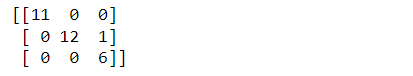
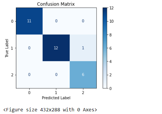
檢視模型的confusion matrix，從結果可看出僅有一個樣本預測錯誤。

from sklearn.metrics import confusion_matrix, classification_report
cm = confusion_matrix(y_test,prediction)
print(cm)

confusion matrix視覺化

import matplotlib.pyplot as plt
from sklearn.metrics import plot_confusion_matrix
 
color = 'black'
matrix = plot_confusion_matrix(classifier, x_test, y_test, cmap=plt.cm.Blues)
matrix.ax_.set_title('Confusion Matrix', color=color)
plt.xlabel('Predicted Label', color=color)
plt.ylabel('True Label', color=color)
plt.show()

最後，呼叫classification_report即可輸出準確率、精確率、召回率以及F1-score

report = classification_report(y_test, prediction)
print(report)

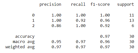
最後一行的support指的是每個類別擁有的總樣本數。

程式碼已上傳至我的Github

參考資料

• How to use Confusion Matrix in Scikit-Learn (with Example)
• 分類器評估方法 — ROC曲線、AUC、Accuracy、PR曲線
• 秋庭伸也, 2020, 零基礎入門的機器學習圖鑑, ISBN:9789865072414

感謝您的瀏覽，我們明天見!