前言

昨天有介紹PCA的降維和分群應用，那這邊再提一下PCA和分群方法有什麼不同。

首先， PCA 和各種「分群」都是屬於非監督是學習的機器學習方法，但是:

• PCA 主要目標還是在降維。它會去計算出主成分，這些主成分的目標是希望能有足夠的代表性去解釋資料，由於前幾個主成分的解釋力就已經很強，十分具有資料代表性了，因此可以選擇較少的主成分數取代維度很大的資料集，進而達到降維的效果。
  PCA的分群比較像是進一步的應用，如果單做 PCA ，它本身並有分群效果。

PCA looks to find a low-dimensional representation of the observations that explain a good fraction of the variance.

• 分群( Clustering )是從資料集(Observations)中找出有同質性的資料們，並把它們分成子群( Subgroup, Partitional )。越相近的資料會被分成同一子群。

Clustering looks to find homogeneous subgroups among the observations

今天主要想介紹的是「分群 Clustering」的機器學習方法，K-means。

分群( Clustering Methods )

• K-means clustering
  • K 值的選擇
  • [R code]
  • [R code] NCI60 data資料應用
• [補充] K-medoids
  • 比較 K-means 、 K-medoids

K-means clustering

K-means 是一種分群的方法，假設今天我們不知道這筆資料集內各資料分別是什麼類別，我們想將整個資料大致分成 K 類/群 時，可以使用 K-means 分群方法。

K-means 分群的計算想法是希望「群內的變異」要盡可能的小。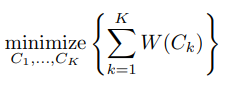

想計算變異量時，常常會透過計算squared Euclidean distance進行數值量化。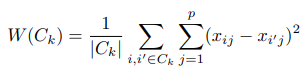

演算法流程:

1. 首先，決定好要將資料分成 K 群 (決定 K 值)。
   ⇒ [圖例 K=3]
2. 將資料隨機指派到群/組別 [step 1] ，並計算各群的中心點 [Iteration 1, step 2a]。
   ⇒ 這時中心點們會很靠近、甚至重疊。
3. 將資料重新分派至最近的中心點的那一群 [step 2b] 。
4. 重新計算新一輪資料群們各自的中心點 [Iteration 2, step 2a]。
5. 重複步驟3、4。 (⇒ 重新分派群組。計算中心點。)
   直到停止改變資料的分群情況為止 [Final Result]。
   

• K 值的選擇

  • 直接估計選擇 ((n/2)^(1/2)，樣本數除2開根號)
  • 手肘法 Elbow Method
    SSE（sum of the squared errors，誤差平方和）作為指標，用 (K, SSE) 作圖，選擇斜率轉折點(陡峭轉平緩)為 K 值。
  • 輪廓係數法 Silhouette Coefficient
  • Canopy (結合 Elbow Method 、 Silhouette Coefficient )

• [R code]

使用的 kmeans( data, k, nstart )函式進行 K-means 分群。

nstart 指的是嘗試 n 種隨機配置生成的初始中心，提供最佳初始中心。
建議設置 20 或 50 ，至少有一定的大小，不要設 1 。

由於二維資料比較容易以圖形展現結果，這邊示範將隨機生成的二維資料(X) 分群。

## 隨機生成 50 筆二維資料(X)
set.seed (2)
x <- matrix ( rnorm (50 * 2), ncol = 2)
x[1:25, 1] <- x[1:25, 1] + 3
x[1:25, 2] <- x[1:25, 2] - 4

         [,1]      [,2]
[1,] 2.103085 -4.838287
[2,] 3.184849 -1.933699
[3,] 4.587845 -4.562247
[4,] 1.869624 -2.724284
[5,] 2.919748 -5.047573
[6,] 3.132420 -5.965878
...

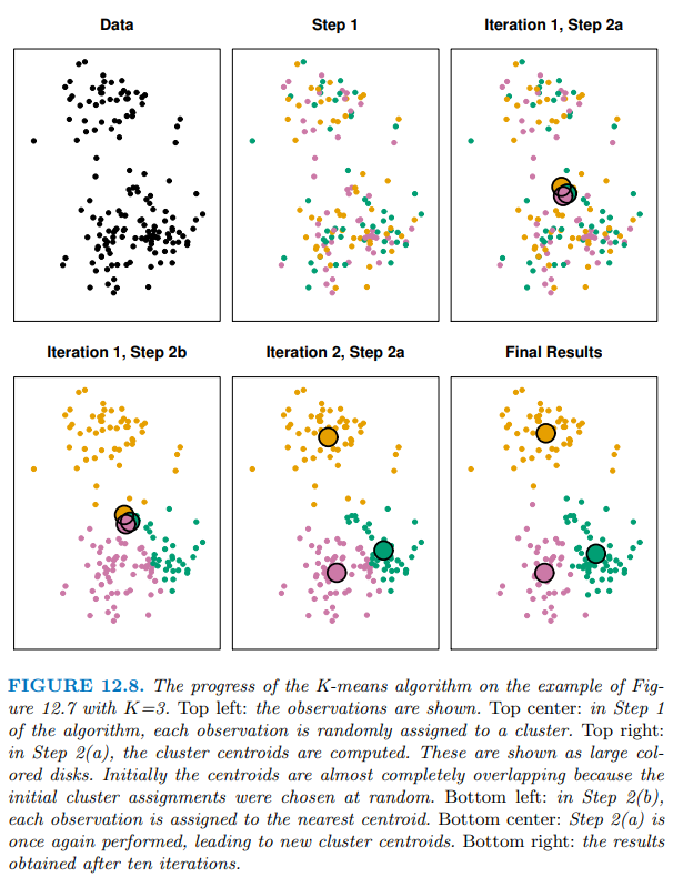
分成兩群(k=2):

km.out <- kmeans (x, 2, nstart = 20)
km.out$cluster # 分群結果,分成哪群

plot (x, col = (km.out$cluster + 1),
        main = "K- Means Clustering Results with K = 2",
        xlab = "", ylab = "", pch = 20, cex = 2)

> km.out
K-means clustering with 2 clusters of sizes 25, 25

Cluster means:
        [,1]       [,2]
1  3.3339737 -4.0761910
2 -0.1956978 -0.1848774

Clustering vector:
 [1] 1 1 1 1 1 1 1 1 1 1 1 1 1 1 1 1 1 1 1 1 1 1 1 1 1 2
[27] 2 2 2 2 2 2 2 2 2 2 2 2 2 2 2 2 2 2 2 2 2 2 2 2

Within cluster sum of squares by cluster:
[1] 63.20595 65.40068
 (between_SS / total_SS =  72.8 %)

Available components:

[1] "cluster"      "centers"      "totss"       
[4] "withinss"     "tot.withinss" "betweenss"   
[7] "size"         "iter"         "ifault"

km.out$tot.withinss: Total within-cluster sum of squares.(整體資料的 sum of squares)
km.out$withinss : The individual within-cluster sum-of-squares.(各群內分別的 sum of squares)

> km.out$tot.withinss
[1] 128.6066
> km.out$withinss
[1] 63.20595 65.40068

分群結果:

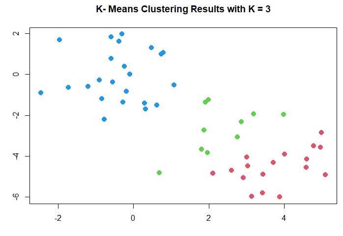
分成三群(k=3):

km.out <- kmeans (x, 3, nstart = 20)
km.out
plot (x, col = (km.out$cluster + 1),
      main = "K- Means Clustering Results with K = 3",
      xlab = "", ylab = "", pch = 20, cex = 2)

• [R code] NCI60 data資料應用
  使用 NCI60 data 示範 k-means 分群，
  以 pc1、pc2、pc3 為軸做圖視覺化呈現 k-means分群(4群)的結果，並對照真實cancer types。

# NCI60 data
library (ISLR2)
nci.labs <- NCI60$labs
nci.data <- NCI60$data
dim(NCI60$data)
table(nci.labs )
dim(iris)

# 標準化資料scale the data
sd.data <- scale(nci.data)

## k-means 分群(clustering)
set.seed (2)
km.out <- kmeans (sd.data, 4, nstart = 20) # 4 cluster
km.clusters <- km.out$cluster # 得到分群結果

## PCA 
pr.out <- prcomp (nci.data , scale = TRUE)

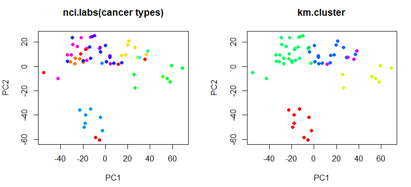
# 在 pc1, pc2 axis上呈現k-means分群結果 (對照真實cancer types)
par (mfrow = c(1,  2))
Cols <- function (vec) {
  cols <- rainbow ( length ( unique (vec)))
  return (cols[as.numeric (as.factor (vec))])
}

# show cluster on pc1, pc2 axis
plot (pr.out$x[, c(1, 2)], col = Cols (nci.labs), pch = 19,
       main = "nci.labs(cancer types)")
plot (pr.out$x[, c(1, 2)], col = Cols(km.clusters), pch = 19,
       main = "km.cluster")

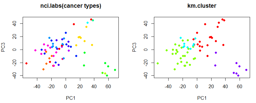
# show cluster on pc1, pc3 axis
plot (pr.out$x[, c(1, 3)], col = Cols(nci.labs), pch = 19,
      main = "nci.labs(cancer types)")
plot (pr.out$x[, c(1, 3)], col = Cols (km.clusters), pch = 19,
      main = "km.cluster")

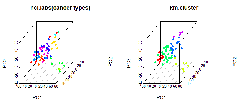
# 3d plot
# install.packages("scatterplot3d")
library(scatterplot3d)
scatterplot3d(pr.out$x[, c(1,2,3)], pch = 16, color = Cols(nci.labs), main = "nci.labs(cancer types)")
scatterplot3d(pr.out$x[, c(1,2,3)], pch = 16, color = Cols(km.clusters), main = "km.cluster")

[補充] K-medoids

K-medoids 也是一種分群的非監督是機器學習方法，和 K-means 不同， 分群計算迭代時不是計算平均值，而是計算群中的 medoid，計算距離並非用 Euclidean distance，而是去計算兩兩(樣本、中心)之間的距離和。

K-medoids 演算法: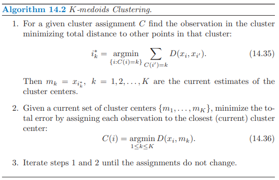

• 比較 K-means 、 K-medoids 兩者差異:

參考資料、網站、書籍

An Introduction to Statistical Learning with Applications in R. 2nd edition. Springer. James, G., Witten, D., Hastie, T., and Tibshirani, R. (2021).

The Elements of Statistical Learning: Data Mining, Inference, and Prediction. 2nd edition. Springer. Hastie, T., Tibshirani, R. and Friedman, J. (2016).

[機器學習首部曲] 聚類分析 K-Means / K-Medoids (@PyInvest)
https://pyecontech.com/2020/05/19/k-means_k-medoids/

E.M. Mirkes, K-means and K-medoids applet. University of Leicester, 2011.
http://www.math.le.ac.uk/people/ag153/homepage/KmeansKmedoids/Kmeans_Kmedoids.html