決策樹 (Decision Tree) 是種簡單好懂且被廣泛使用的分類器,為監督式學習的方法。通過訓練資料構建決策樹,可以對未知的新資料進行分類。
分類模型示意圖: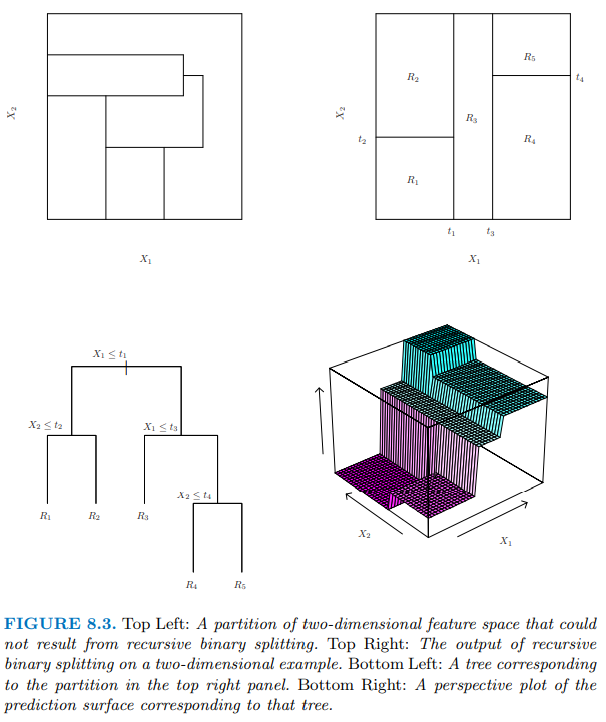
一棵決策樹的架構大致上長這樣: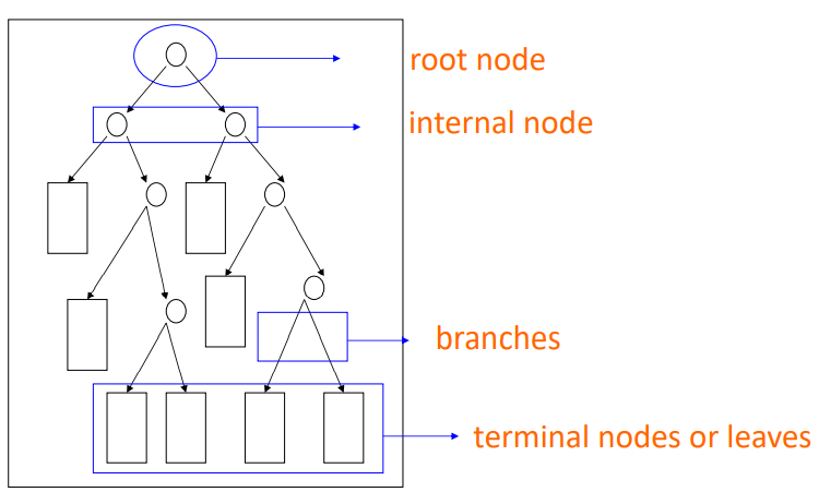
一棵決策樹類會有:
常見的決策樹演算法有這三種,分別是依據不同的量化特徵值去建構決策樹的節點判斷依據:
接下來主要要講的是 CART (Classification And Regression Trees) 決策樹。
CART每次都會選擇當前資料集中具有最小 Gini 資訊增益的特徵作為結點劃分決策樹。
衡量出資料集某個特徵所有取值的 Gini index 後,就可以得到該特徵的Gini Split info,也就是Gini Gain。
不考慮剪枝情況下,分類決策樹遞迴建立過程中就是每次選擇 GiniGain 最小的節點做分叉點,直到子資料集都屬於同一類或者所有特徵用光了。
Gini值越小,表示樣本的純淨度越高(該樣本只屬於同一類的機率越高),越大則代表類別的不確定性越大。
當樹建得太複雜時,會發生overfit資料的情形,這時我們可以選擇去剪枝。
以下簡單說明一下剪枝的概念:
剪枝就是在最小化RSS時,RSS的計算會加入一個樹複雜度的懲罰項complexity penalty(alpha),樹的節點數目為 T ,得到一個 Tree Scroe: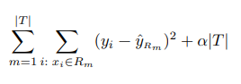
經由 Cost complexity pruning 可以得到一群alpha值。complexity parameter (alpha) 數值集合的計算是透過樹複雜度的組合(j 個 alpha值)乘上(與對應的 j 棵樹的複雜度 terminal nodes: T )去計算 test error 得到不同節點數目的樹對應到的 complexity parameter (alpha) 值。
剪枝的方法是從 training data 裡使用 k fold cross validation ,每折計算出一群 complexity parameter (alpha) 數值集合,找到 SSR (Sum of Square Residual) 最低的樹與其對應的alpha。
重複計算並記錄了 k 個 alpha,表現最好(出現次數最多)的alpha會被定為最終alpha值,所對應的 T 終點節點數也會是最終決定減枝的節點數目。
詳細說明可以參閱:Minimal Cost-Complexity Pruning
想要在 R 裡建立 CART Tree 時,可以使用rpart套件建立模型,接著使用rpart.plot套件視覺化模型和分類/預測結果。
rpart (formula = Y~X, data, method, control)
#install.packages("rpart")
#install.packages("rpart.plot")
library(rpart)     # For decision tree model
library(rpart.plot)# For data visualization


## 決策樹的限制
rpart.control<- rpart.control(
    minsplit  = minsplit, #每一個node最少要幾個data。
    minbucket = minbucket, #在末端的node上最少要幾個data。
    cp    = cp, #complexity parameter。
    maxdepth  = maxdepth #Tree的深度。
 ... )
## 建立模型
fit.treemodel<- rpart(method  = ‘class’ /‘anova’, #(Classification tree 類別Y)/ (Regression tree     連續Y)。
       control = rpart.control。 # 決策樹的限制
        ... )
使用prune()可以去進行樹的剪枝:
# Prune the tree with the best cp value (the lowest cross-validation error-xerror)
bestcp <-fit.treemodel$cptable[which.min(fit.treemodel$cptable[,"xerror"]),"CP"]

pruned.c.tree <- prune(fit.c.tree, cp = bestcp)
套件rpart的詳細說明。
Classification Tree 是由最小化 Classification error rate, Gini index, Cross-entropy 去建立節點,並建構樹模型: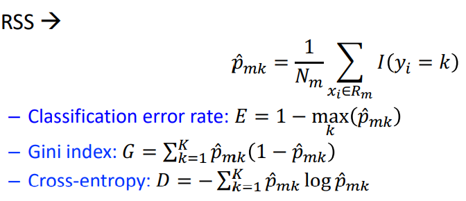
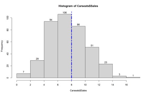
這邊以套件ISLR的 Carseats dataset 建立分類問題,新增一個分類變數"High(Sales>8)",可以去分類哪類的店家會有比較高的銷售量。
資料中含有400(stores)筆觀察值, 11 個變量,我們有興趣的目標為Sales(銷售單位/千人)。
library(ISLR)      # Carseats data set
## 觀察資料型態---------------------------------------------------------------
data(Carseats)
names(Carseats)   #資料裡,各變數名稱
dim(Carseats)     #資料筆數, 變數數量
str(Carseats)     #列出資料內每個欄位的狀態
summary(Carseats) #連續型資料:會看到 Qu.  #類別型資料:會看到不同數值的資料個數
head(Carseats)    #呈現前6筆資料

# 畫Histogram觀察Sales
h<-hist(Carseats$Sales,xaxt = "n")
text(h$mids,h$counts,labels=h$counts, adj=c(0.5, -0.5))
axis(1, at = seq(round(min(Carseats$Sales)),
                +round(max(Carseats$Sales)),by=2))
abline(v = 8, col = "blue", lwd = 4, lty = 4)

# Creates a new binary variable, High.
Carseats.H<-Carseats
Carseats.H$High = ifelse(Carseats.H$Sales <=8,"No_Low","Yes_High")
Carseats.H$High<-as.factor(Carseats.H$High) # Code "High" as a factor variable.
class(Carseats.H$High)
Carseats.H <- Carseats.H[,-1]               # Remove the variable, Sales.

# Data partition
# 50% dataset used for training purposes and 50% used for testing purposes.
set.seed(234)
train = sample(1:nrow(Carseats.H), size=ceiling(0.5*nrow(Carseats.H)))
Carseats.train=Carseats.H[train,]
Carseats.test=Carseats.H[-train,]
分類哪類的店家會有比較高的銷售量(High: Sales>8 ,分為Yes/ No)。
library(rpart)     # For decision tree model
library(rpart.plot)# For data visualization

fit.c.tree = rpart(High ~ ., data=Carseats.train, method = "class", cp=0.008)
fit.c.tree

# rpart.control寫在外面的寫法
ct <- rpart.control(cp=0.008)
fit.c.tree2 = rpart(High ~ ., data=Carseats.train, method = "class", control=ct)
fit.c.tree2


# Visualizing the unpruned tree
prp(fit.c.tree,         # 模型
    faclen=0,           # 呈現的變數不要縮寫
    extra=2,            # no. correct classifications / no. observations in that node
    box.palette="auto") #color palette
#?prp()                 # 參考更多畫圖指令

# Checking the order of variable importance 分類時的重要特徵變數
fit.c.tree$variable.importance

# Predict Using the Classification Tree
pred.c.tree = predict(fit.c.tree, Carseats.test, type = "class")
table(pred.c.tree, Carseats.test$High)
> fit.c.tree
n= 200

node), split, n, loss, yval, (yprob)
      * denotes terminal node

 1) root 200 90 No_Low (0.55000000 0.45000000)
   2) ShelveLoc=Bad,Medium 154 52 No_Low (0.66233766 0.33766234)
     4) Price>=92.5 132 35 No_Low (0.73484848 0.26515152)
       8) Advertising< 13.5 106 19 No_Low (0.82075472 0.17924528) *
       9) Advertising>=13.5 26 10 Yes_High (0.38461538 0.61538462)
        18) Age>=44 15  6 No_Low (0.60000000 0.40000000) *
        19) Age< 44 11  1 Yes_High (0.09090909 0.90909091) *
     5) Price< 92.5 22  5 Yes_High (0.22727273 0.77272727) *
   3) ShelveLoc=Good 46  8 Yes_High (0.17391304 0.82608696)
     6) Price>=135 7  2 No_Low (0.71428571 0.28571429) *
     7) Price< 135 39  3 Yes_High (0.07692308 0.92307692) *
> fit.c.tree$variable.importance
  ShelveLoc       Price Advertising         Age   CompPrice      Income
 16.8994918  14.5382371   8.5411152   3.2895105   1.7804529   1.4952320
  Education  Population
  0.5980928   0.2990464

> table(pred.c.tree, Carseats.test$High)

pred.c.tree No_Low Yes_High
   No_Low      110       32
   Yes_High     16       42
loss:如果將節點的預測類應用於所有行,則這是將被錯誤分類的總行數
Yval: 分類出來大多是哪類mean response value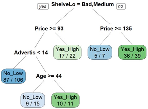
printcp(fit.c.tree) #cross-validated error rate
plotcp(fit.c.tree)
# Prune the tree with the best cp value (the lowest cross-validation error-xerror)
bestcp <-fit.c.tree$cptable[which.min(fit.c.tree$cptable[,"xerror"]),"CP"]

pruned.c.tree <- prune(fit.c.tree, cp = bestcp)
prp(pruned.c.tree,faclen=0,extra=2, box.palette="auto")

# Predict Using the Classification Tree
pred.pruned.c.tree = predict(pruned.c.tree, Carseats.test, type = "class")
table(pred.pruned.c.tree, Carseats.test$High)
sum(diag(table(pred.pruned.c.tree, Carseats.test$High))/200) #準確率
> printcp(fit.c.tree)
Classification tree:
rpart(formula = High ~ ., data = Carseats.train, method = "class",
    cp = 0.008)
Variables actually used in tree construction:
[1] Advertising Age         Price       ShelveLoc

Root node error: 90/200 = 0.45
n= 200
        CP nsplit rel error  xerror     xstd
1 0.333333      0   1.00000 1.00000 0.078174
2 0.133333      1   0.66667 0.66667 0.072008
3 0.066667      2   0.53333 0.60000 0.069761
4 0.033333      3   0.46667 0.54444 0.067582
5 0.008000      5   0.40000 0.66667 0.072008
prune tree "cp (complexity parameter)"的選擇方法 ,是去選擇cv中對應到最小的test error 的cp。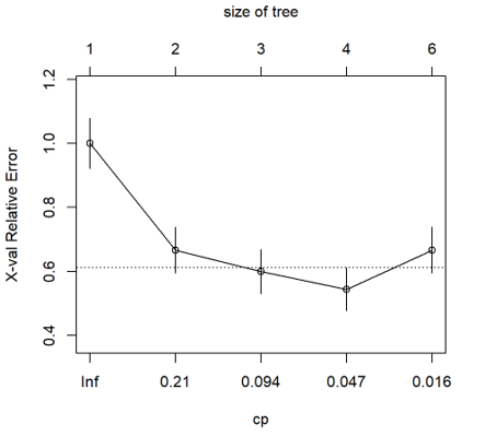
最終的 prune tree: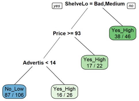
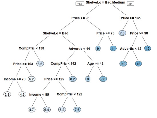
Regression Tree 建立的方法是去最小化 RSS: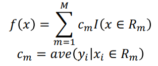
這邊同樣以套件ISLR的 Carseats dataset 做示範,以Sales (銷售單位/千人) 這個連續變數做為目標,去建構的Regression tree 的預測問題。
library(rpart)     # For decision tree model
library(rpart.plot)# For data visualization

Carseats.S <- Carseats
# Data partition
set.seed(234)
train = sample(1:nrow(Carseats.S), size=ceiling(0.5*nrow(Carseats.S)))
Carseats.train=Carseats.S[train,]
Carseats.test=Carseats.S[-train,]


# Build the regression tree on the training set
fit.r.tree = rpart(Sales ~ ., data=Carseats.train, method="anova", cp=0.008)
fit.r.tree
prp(fit.r.tree,faclen=0, box.palette="auto")

fit.r.tree$variable.importance

# Predict Using the Regression Tree
pred.tree = predict(fit.r.tree, Carseats.test)
# Calculate the mean square error 迴歸樹的 error 是去計算 mean square error
mse <- mean((pred.tree - Carseats.test$Sales)^2)
mse
## Pruning the tree
# Finding the best CP value
# Prune the Regression tree with the best cp  value
# (the lowest cross-validation error - xerror)
printcp(fit.r.tree)
plotcp(fit.r.tree)
bestcp <- fit.r.tree$cptable[which.min(fit.r.tree$cptable[,"xerror"]),"CP"]

pruned.r.tree <- prune(fit.r.tree, cp = bestcp)
prp(pruned.r.tree, box.palette="auto")

# Checking the order of variable importance
pruned.r.tree$variable.importance


# Use the test data to evaluate performance of pruned regression tree
pred.pruned.r.prune = predict(pruned.r.tree, Carseats.test)
# Calculate the MSE for the pruned tree
pruned.mse <- mean((pred.pruned.r.prune - Carseats.test$Sales)^2)
pruned.mse
優點
分類依據簡單好懂,容易視覺化模型及分類結果,建模速度快。
缺點
決策樹很容易有「Overfitting(過度擬合)」的問題。因此我們可以做一些限制或是剪枝避免Overfitting的產生。
| 限制 | 意思 |
|---|---|
| Minimum samples for a node split | 資料數目(samples)至少多少才能產生一個判斷節點。 |
| Minimum samples for a terminal node | 每個最末節點(葉子)至少要有多少資料數目(samples)。 |
| Maximum depth of tree | 決策樹的深度(最多做幾次判斷)。 |
| Maximum number of terminal nodes | 最末節點(葉子)數目。 |
| Maximum features to consider for split | 在節點上,做判斷依據時最多使用多少特徵變數。 |
統計與機器學習 Statistical and Machine Learning, 台大課程. 王彥雯 老師.
An Introduction to Statistical Learning with Applications in R. 2nd edition. Springer. James, G., Witten, D., Hastie, T., and Tibshirani, R. (2021).
決策樹(Decision Tree)常見的三種算法(ID3、C4.5、CART)(@Roger Yong)
https://roger010620.medium.com/%E6%B1%BA%E7%AD%96%E6%A8%B9-decision-tree-%E5%B8%B8%E8%A6%8B%E7%9A%84%E4%B8%89%E7%A8%AE%E7%AE%97%E6%B3%95-id3-c4-5-cart-54091ca85044
Minimal Cost-Complexity Pruning
https://online.stat.psu.edu/stat508/lesson/11/11.8/11.8.2
Tree-Based Methods
https://afit-r.github.io/tree_based_methods


 iThome鐵人賽