caret套件中的 隨機森林 模型Random forest 隨機森林是決策樹的一種延伸方法,它可以提高準確率,也能同時避免建立決策樹時容易出現的overfitting。除此之外,當資料的解釋變數們有共線性(Collinearity)或類別不平衡(Class Imbalance)的問題時,隨機森林是很好的模型選擇。
隨機森林的概念就是隨機抽取部份樣本以及抽取一部份的解釋變數(X),去建立一棵樹的模型,重複建立了多棵的樹,他們組合起來時也就形成隨機森林的模型。
隨機森林演算法: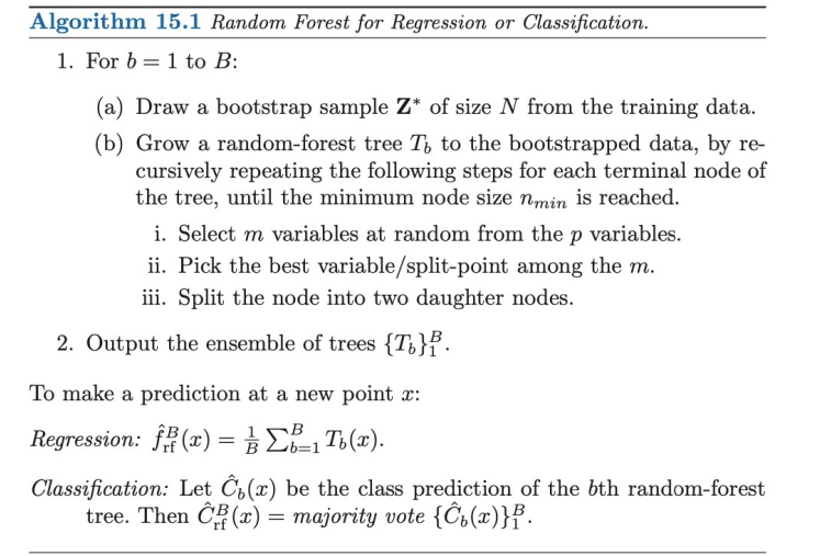
隨機森林是以決策樹為基礎建立模型,所以理所當然能處裡分類也能處理預測問題。
在建立隨機森林的模型時,我們要挑選的重要變數包含:
ntree,決定生成多少棵決策樹。mtry,決定抽取多少個多少個變數去建每棵決策樹。在 R 裡建立隨機森林時,可以使用randomForest套件建立模型,建立的隨機森林模型和決策樹模型一樣可以對新資料進行分類、預測結果。
基本函式:randomForest(Y~X, data, subset, na.action=na.fail)。
#install.packages("randomForest")
library(randomForest)

randomForest(formula = Y~X,
    subset   = training_data_index,# 注意! 這裡不是直接放入training data,而是index值
    na.action  =‘na.fail’,# (默認值), 不允許資料中出現遺失值/ ‘na.omit’,刪除遺失值。
    importance = TRUE,# 结合importance()函数使用,用來觀察重要變數。
    ntree   = num_tree,# number of trees, RF裡生成的決策樹數目。
    mtry    = m_variables_try, # 每次抽樣時需要抽「多少個變數」,
                               # 建議設置 ?/3  (Regression trees);  √?(Classification trees)
    sampsize  = sampsize,#訓練每棵樹模型的樣本數大小。預設是使用63.25%訓練資料集的比例。
    nodesize  = nodesize,# 末梢(葉)節點最小觀察資料個數。
    Maxnode  = Maxnode,# 內部節點最大個數值。
    ... )
| 參數設定 | 意思 | 說明 |
|---|---|---|
| ntree | RF裡生成的決策樹數目。number of trees. | 我們希望有足夠的樹來穩定模型的誤差,但過多的樹會是沒效率且沒必要的,特別是遇到大型資料集的時候。 |
| mtry | 建每棵樹,抽樣時需要抽「多少個變數」。 | 建議設置 p/3 (迴樹樹Regression trees); √p(分類樹Classification trees)。 |
| sampsize | 訓練每棵樹模型的樣本數大小。 | 預設是使用63.25%訓練資料集的比例。 |
| nodesize | 訓練的每棵樹時,末梢(葉)節點最少要有多少觀察資料個數。 | 控制模型複雜度的變數。末梢(葉)節點需含有的資料量越大,生成的樹越簡化/越淺。 |
| maxnode | 每棵樹的內部節點最多只能有多少節點。 | 控制模型複雜度的變數。內部節點越多,生成的樹越複雜/越深。 |
mtry
假設資料整體總共有 p 個變數。
隨機森林設定 mtry = p 時,代表每次(棵樹)都抽取所有特徵變數去建樹,因此 randomForest()建構出的是一棵 Bagging trees。Bagging tree 的手法僅能助於降低 variance。
設定 mtry = 1,會造就每一次split所使用的變數completely random,每個變數都有機會但會造成非常偏差的結果。
sampsize
sampsize 為訓練每棵樹模型的樣本數大小。預設是使用63.25%訓練資料集的比例,因為這個是獨立觀察值出現在bootstrapped sample的期望機率值。較低的樣本數大小雖然會降低訓練時間,但可能會產生不必要的偏差(biased)。增加樣本數大小可以提升模型正確率,但有可能會產生overfitting(因為會增加模型變異性 (variance))。所以一般來說,sampsize 會使用60-80%的比例。
nodesize, maxnode
都是樹生長深度(複雜度)的一種限制方式。當樹長得越深時,模型變異性愈高,有過度配適的風險;當樹長得越淺時則會有較多偏差,可能沒辦法完整捕捉資料中的特性。
[補充] R 中對應的套件randomForest詳細說明。
Boston dataset實例示範 Bagging trees、隨機森林 Random Forest Regression Example。
這邊打算去預測房價中位數medv:
## 載入、觀察 Boston dataset
library(MASS) #Boston dataset
data('Boston')
dim(Boston)
names(Boston)

set.seed (123)
index.train = sample(1:nrow(Boston), size=ceiling(0.8*nrow(Boston))) # training dataset index
train = Boston[index.train, ] # trainind data
test = Boston[-index.train, ] # test data
#  Bagging trees: All predictors should be considered for each split of the tree.
library(randomForest)
bag.boston <- randomForest (medv ~ ., data = Boston ,
                            subset = index.train ,
                            mtry = ncol(Boston)-1, # 14variables - 1(medv)=13
                            importance = TRUE)
bag.boston

# Perform on the test set
test <- Boston[-index.train  , ]
yhat.bag <- predict (bag.boston , newdata = Boston[-index.train , ])
plot (yhat.bag , test$medv)
abline (0, 1)
mean ((yhat.bag - test$medv)^2) #MSE
因為這裡是 Regression trees 所以一開始嘗試選擇mtry時會建議選擇 p/3 variables。
library(randomForest)
rf.boston <- randomForest (medv ~ ., data = Boston ,
                           subset = index.train ,
                           mtry = 4,           #13/3
                           importance = TRUE)
rf.boston
接著我們可以試著挑選參數,首先從ntree 開始挑選,選擇RF要建立幾棵樹:
## Observe that what is the best number of trees(ntree)
plot(rf.boston) # MSE on OOB samples (OOB error)
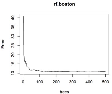
可以看到ntree=200左右,模型的平均誤差OOB(out-of-bag)MSE 穩定平緩,所以選擇ntree=200。
接著使用 tuneRF(x.train.data, y.train.data, ntree),來tune mtry,決定抽取多少個多少個變數去建每棵決策樹。。
# x.train.data= train[,-14]= training data without Y(medv)
# y.train.data=train[,14]= Y(medv)
tuneRF(x=train[,-14], y=train[,14],
       ntreeTry= 200)
> set.seed (123)
> tuneRF(x=train[,-14], y=train[,14],ntreeTry= 200)
mtry = 4  OOB error = 10.28749
Searching left ...
mtry = 2 	OOB error = 12.95853
-0.2596396 0.05
Searching right ...
mtry = 8 	OOB error = 10.3901
-0.009974117 0.05
  mtry OOBError
2    2 12.95853
4    4 10.28749
8    8 10.39010
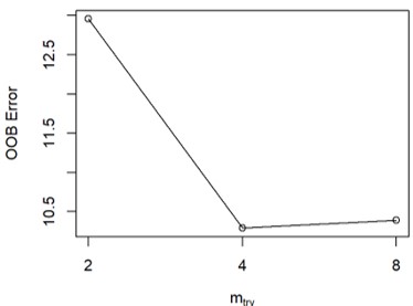
選擇OOB(out-of-bag)erro 最低的mtry=4。
所以我們的最終模型為:
##最終模型
# Set mtry=4, ntree=200 to build the model.
rf.tune.boston <- randomForest (medv ~ ., data = Boston ,
                           subset = index.train ,
                           mtry = 4,
                           ntree = 200,
                           importance = TRUE)
rf.tune.boston

## 預測結果
yhat.tune.rf <- predict (rf.tune.boston, newdata = test)
mean ((yhat.tune.rf - test$medv)^2)#MSE
> rf.tune.boston

Call:
 randomForest(formula = medv ~ ., data = Boston, mtry = 4, ntree = 200,      importance = TRUE, subset = index.train)
               Type of random forest: regression
                     Number of trees: 200
No. of variables tried at each split: 4

          Mean of squared residuals: 11.14222
                    % Var explained: 86.77
> yhat.tune.rf <- predict (rf.tune.boston, newdata = test)
> mean ((yhat.tune.rf - test$medv)^2)#MSE
[1] 12.0481
建完模型後,我們可以看看什麼是比較重要的變數:
# Importance of each variable
importance (rf.tune.boston)        # %Increase in MSE(); Increase in node purity
importance (rf.tune.boston,type=1) # %IncMSE
varImpPlot (rf.tune.boston)
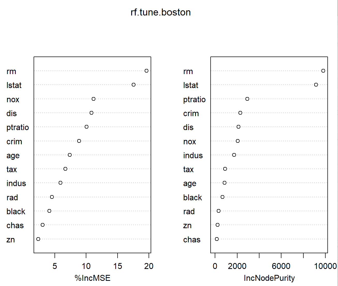
可以看出house size (rm) 和 The wealth of the community (lstat)是最重要的兩個影響預測的變數。
顯示variable importance,也就是解釋變數們對損失函數(Loss Function)的貢獻。
> importance (rf.tune.boston)        # %Increase in MSE(); Increase in node purity
          %IncMSE IncNodePurity
crim     8.885338     2293.4591
zn       2.382149      234.1868
indus    5.930444     1723.8176
chas     3.088354      169.4439
nox     11.159399     2051.2330
rm      19.630168     9817.5530
age      7.412050      850.4205
dis     10.846649     2128.9522
rad      4.545620      322.4924
tax      6.686760      918.5644
ptratio 10.059433     2926.1168
black    4.147858      673.1858
lstat   17.545261     9148.7841
%IncMSE(Mean Decrease Accuracy)可以得知去除這項解釋變數(X)的話,模型的準確率會減少幾%。
library(randomForest)
data("iris")
names(iris)
dim(iris)
sqrt(5)
set.seed(123)
index.train.iris = sample(1:nrow(iris), size=ceiling(0.8*nrow(iris)))
train.iris = iris[index.train.iris, ]
test.iris = iris[-index.train.iris, ]

rf.iris<-randomForest(Species~.,  data=iris, subset=index.train.iris)
plot(rf.iris,lwd=2)

#Important variables
importance(rf.iris) # MeanDecreaseGini
varImpPlot(rf.iris, sort = TRUE)

## Perform on the testing data
# predict()
# type: response(預測的分類), prob(預測分為各種類的機率), vote(預測時各分類的獲得的投票數)
predict(rf.iris, test.iris, type="response")
predict(rf.iris, test.iris, type="prob")
predict(rf.iris, test.iris, type="vote")

iris.pred <- predict(rf.iris, test.iris) # 預設為type="response"
iris.pred

table(observed=test.iris$Species , predicted = iris.pred) # Confusion matrix
mean(test.iris$Species==iris.pred) # Accuracy
ntrees 對上 OOB(out-of-bag) Erro Rates: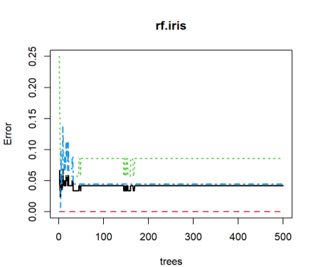
在分類樹上,可以顯示出對於各目標類別(Y)的分類誤差。
以上圖舉例,黑色實線表示整體的 OOB Error rate,而其他顏色虛線表示各類別的 OOB Error Rate。
Important variables: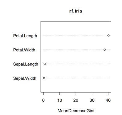
在這項個隨機森林分類模型裡,Petal.Length、Petal.Width 是相對比較重要的分類依據。
> importance(rf.iris) # MeanDecreaseGini
             MeanDecreaseGini
Sepal.Length         0.8486603
Sepal.Width          0.3728377
Petal.Length        40.1408059
Petal.Width         37.8613906
MeanDecreaseGini(Mean Decrease Gini, IncNodePurity)可以得知使用這項解釋變數(X)去分類判斷時,Gini 係數減少的平均值。
Gini係數值越小,表明樣本的純淨度越高(即該樣本只屬於同一類的概率越高),越大則代表不確定性越大。
caret套件中的 隨機森林 模型使用caret套件中,train( )函式, 設定method = "ranger",也可以去建立隨機森林模型。caret套件可以用來建很多不同的模型。
caret會tune 3個超參數:
mtry
splitrulemin.node.size
以下為補充,程式碼網頁來源(by Michael Foley)
## packages for builiding models
library(caret)  # for workflow
library(tidyverse)
library(skimr)  # neat alternative to glance + summary
## Dataset
library(ISLR)  # For OJ datasets

set.seed(12345)
partition <- createDataPartition(y = oj_dat$Purchase, p = 0.8, list = FALSE)
oj.train <- oj_dat[partition, ]
oj.test <- oj_dat[-partition, ]
rm(partition)

## RF model
oj.frst = train(Purchase ~ .,
               data = oj.train,
               method = "ranger",  # for random forest
               tuneLength = 5,  # choose up to 5 combinations of tuning parameters
               metric = "ROC",  # evaluate hyperparamter combinations with ROC
               trControl = trainControl(
                 method = "cv",  # k-fold cross validation
                 number = 10,  # 10 folds
                 savePredictions = "final",       # save predictions for the optimal tuning parameter1
                 classProbs = TRUE,  # return class probabilities in addition to predicted values
                 summaryFunction = twoClassSummary  # for binary response variable
                 )
               )
## predict result
oj.pred <- predict(oj.frst, oj.test, type = "raw")
oj.conf <- confusionMatrix(data = oj.pred,
                            reference = oj.test$Purchase)
oj.conf

oj.frst.acc <- as.numeric(oj.conf$overall[1])
rm(oj.pred)
rm(oj.conf)
#plot(oj.bag$, oj.bag$finalModel$y)
#plot(varImp(oj.frst), main="Variable Importance with Simple Classication")
## Dataset
library(ISLR)  # For OJ, and Carseats datasets

set.seed(12345)
partition <- createDataPartition(y = carseats_dat$Sales, p = 0.8, list = FALSE)
carseats.train <- carseats_dat[partition, ]
carseats.test <- carseats_dat[-partition, ]


## RF model
carseats.frst = train(Sales ~ .,
               data = carseats.train,
               method = "ranger",  # for random forest
               tuneLength = 5,  # choose up to 5 combinations of tuning parameters
               metric = "RMSE",  # evaluate hyperparamter combinations with RMSE
               trControl = trainControl(
                 method = "cv",  # k-fold cross validation
                 number = 10,  # 10 folds
                 savePredictions = "final"       # save predictions for the optimal tuning parameter1
                 )
               )
carseats.frst
plot(carseats.frst)

## predict result
carseats.pred <- predict(carseats.frst, carseats.test, type = "raw")
plot(carseats.test$Sales, carseats.pred,
     main = "Random Forest Regression: Predicted vs. Actual",
     xlab = "Actual",
     ylab = "Predicted")
abline(0, 1)
## RMSE
carseats.frst.rmse <- RMSE(pred = carseats.pred,
                           obs = carseats.test$Sales)
rm(carseats.pred)
#plot(varImp(carseats.frst), main="Variable Importance with Regression Random Forest")
The Elements of Statistical Learning: Data Mining, Inference, and Prediction. 2nd edition. Springer. Hastie, T., Tibshirani, R. and Friedman, J. (2016).
Bagging, Random Forest, and Gradient Boosting using R
(@Michael Foley)
https://rpubs.com/mpfoley73/529130
R筆記 – (16) Ensemble Learning(集成學習)(@skydome20)
https://rpubs.com/skydome20/R-Note16-Ensemble_Learning


 iThome鐵人賽