今日大綱

• 資料集
• 衡量指標
• 程式碼

資料集

今天我以sklearn所提供的資料集舉例，預測加州不同區的房價，獨立變數與依變數的敘述如下:

獨立變數

• MedInc: 收入的中位數
• HouseAge:屋齡的中位數
• AveRooms:每戶平均房間數量
• AveBedrms:每戶平均臥室數量
• Population:人口數
• AveOccup:每戶平均人口數
• Latitude:緯度
• Longitude:經度

依變數

• MedHouseVal:加州行政區的房價中位數，以100,000為一單位

衡量指標

1. 平均絕對誤差 (Mean absolute error, MAE)
   計算實際值與預測值之間的誤差之絕對值平均
   yi後面的變數稱為y head，代表預測值。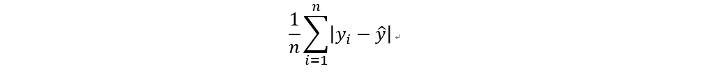
   

2. 均方誤差 (Mean square error, MSE)
   計算實際值與預測值之間的誤差之平方平均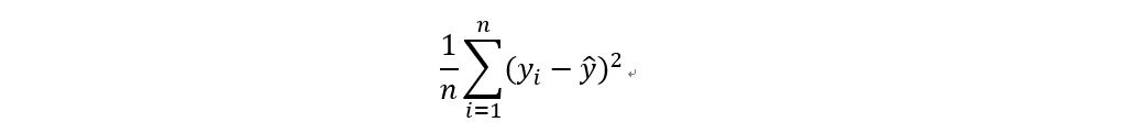
   

3. 均方根誤差 (Root mean square error, RMSE)
   計算實際值與預測值之間的誤差之平方平均，再開根號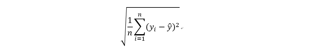
   

4. R平方 (R squared)
   R平方為衡量模型的指標，其介於0到1之間，代表x解釋y的變量的比例，越高代表模型的表現越好。如果R平方等於0.7，表示y(依變數)的70%變化能由x(獨立變數)解釋。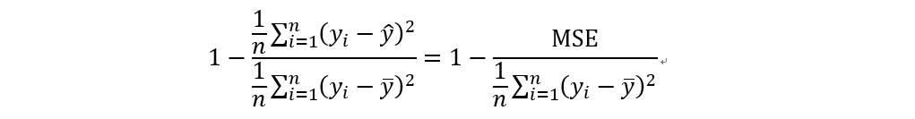
   

程式碼

首先，先匯入將會使用到的libraries，並且將房價資料儲存至data變數中。將data列印出，檢視data裡的資料

from sklearn.datasets import fetch_california_housing
import pandas as pd

data = fetch_california_housing()
print(data)

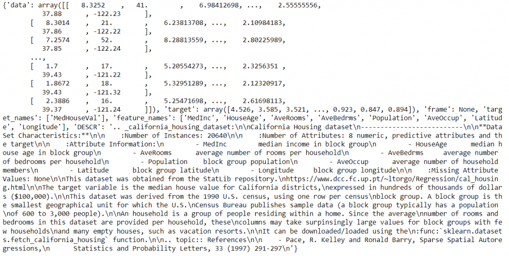
data所抓到的資料型態為字典(dictionary)，target的value就是目標變數，data的value就是獨立變數，將他們儲存成y與x，並且觀察各個特徵的敘述性統計。Pandas的dataframe有個function為describe()，只要打dataframe.describe()就會列出所有連續變數的敘述性統計資料，包含數量、平均數、標準差、最大值、最小值等。

x = pd.DataFrame(data['data'])
#data的feature_names指定成x的column名稱
x.columns = data['feature_names']
y = pd.DataFrame(data['target'])
#data的target_names指定成u的column名稱
y.columns = data['target_names']
print(x.describe(),"\n", y.describe())

結果如下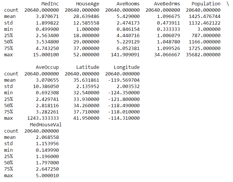

匯入train_test_split將原始資料切割成訓練集(train set)與測試集(test set)，訓練集用來訓練模型，找出最適合描述訓練集資料裡的模型，而測試集用來檢視模型的泛化能力。有時候訓練過度會有過度擬合(overfitting)的問題，有可能因為資料筆數過少，常見的解決方式有正規化(regularization)，加入一個懲罰項，讓某些特徵的權重歸0。

from sklearn.model_selection import train_test_split
from sklearn.linear_model import LinearRegression

x_train, x_test, y_train, y_test = train_test_split(x, y, test_size = 0.2, random_state = 1)
regression = LinearRegression()
regression.fit(x_train, y_train)
y_prediction = regression.predict(x_test)

最後，檢視模型的績效，MAE、MSE；RMSE以及R平方。

from sklearn.metrics import mean_absolute_error,mean_squared_error, r2_score
  
mae = mean_absolute_error(y_test,y_prediction)
#squared True returns MSE value, False returns RMSE value.
mse = mean_squared_error(y_test,y_prediction) #default=True
rmse = mean_squared_error(y_test,y_prediction,squared=False)
r_square = r2_score(y_test, y_prediction)
print("MAE:", round(mae,2), "\nMSE:", round(mse,2), "\nRMSE:", round(rmse,2), "\nR square:", round(r_square,2))

從結果可以發現，R平方為0.6，還有進步的空間。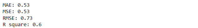

參考文獻

• Evaluation Metrics : 迴歸模型
• 決定係數（R平方）解釋
• [機器學習 ML NOTE]Overfitting 過度學習

感謝您的瀏覽，我們明天見!