今天要來介紹Image Features，並且如何實作特徵選取、人臉辨識，目前影像辨識的支援模組及開放的函式有相當多，所以在實作上可以方便又快速，那我們今天來介紹利用方向梯度直方圖(Histogram of Oriented Gradient, HOG)來提取特徵。

• 一樣匯入先今天範例會用到的模組

%matplotlib inline
import matplotlib.pyplot as plt
import seaborn as sns; sns.set()
import numpy as np

HOG的演算過程：

1. 掃苗所要檢測人形的image
2. 再來將圖片轉換為灰階cmap='gray'
3. 為了降低有些image會因為光線、陰影影響，所以要對圖像進行Gamma校正。Gamma壓縮公式：

   想要了解「伽瑪校正Gamma Correction」內容參考：https://blog.csdn.net/lichengyu/article/details/8457425

4. 將圖像切割數個cell，並統計每個cell的梯度個數
5. 多個cell的特徵值合併，為一個block的HOC 特徵
6. 將所有block的特徵值串聯，為該image的HOG特徵值，這些特徵向量就可以供SVM做分類

from skimage import data, color, feature
import skimage.data

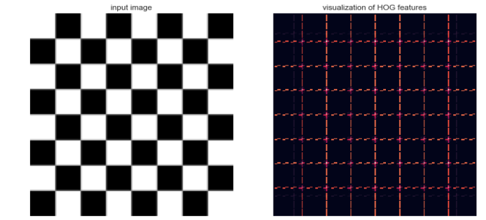
image = color.rgb2gray(data.checkerboard())
hog_vec, hog_vis = feature.hog(image, visualise=True)

fig, ax = plt.subplots(1, 2, figsize=(12, 6),
                       subplot_kw=dict(xticks=[], yticks=[]))
ax[0].imshow(image, cmap='gray')
ax[0].set_title('input image')

ax[1].imshow(hog_vis)
ax[1].set_title('visualization of HOG features');

skimage的相關資料可參考scikit-image：http://scikit-image.org/docs/dev/api/skimage.html

• 在sklearn中，匯入人臉的資料集，可以看到輸出結果，大約有13,000筆訓練資料，作為正面的訓練資料

from sklearn.datasets import fetch_lfw_people
faces = fetch_lfw_people(data='``` 資料路徑 ```'))
positive_patches = faces.images
positive_patches.shape

• 再來匯入在sklearn中，不為人臉的資料集，作為訓練負面的資料

from skimage import data, transform

imgs_to_use = ['camera', 'text', 'coins', 'moon',
               'page', 'clock', 'immunohistochemistry',
               'chelsea', 'coffee', 'hubble_deep_field']
images = [color.rgb2gray(getattr(data, name)())
          for name in imgs_to_use]
          
from sklearn.feature_extraction.image import PatchExtractor

def extract_patches(img, N, scale=1.0, patch_size=positive_patches[0].shape):
    extracted_patch_size = tuple((scale * np.array(patch_size)).astype(int))
    extractor = PatchExtractor(patch_size=extracted_patch_size,
                               max_patches=N, random_state=0)
    patches = extractor.transform(img[np.newaxis])
    if scale != 1:
        patches = np.array([transform.resize(patch, patch_size)
                            for patch in patches])
    return patches

negative_patches = np.vstack([extract_patches(im, 1000, scale)
                              for im in images for scale in [0.5, 1.0, 2.0]])
negative_patches.shape

• 一開始所講解得，檢測人臉最重要的就是提取HOG的特徵值，組合正負兩面的樣本，合併計算HOG的特徵

from itertools import chain
X_train = np.array([feature.hog(im)
                    for im in chain(positive_patches,
                                    negative_patches)])
y_train = np.zeros(X_train.shape[0])
y_train[:positive_patches.shape[0]] = 1
X_train.shape

• 利用之前講解過的SVM，在這裡先用一個簡單得高斯貝氏分類器來會獲取baesline，並利用sklearn中的LinearSVC來更方便的縮放樣本數據的資料

from sklearn.naive_bayes import GaussianNB
from sklearn.cross_validation import cross_val_score
cross_val_score(GaussianNB(), X_train, y_train)

from sklearn.svm import LinearSVC
from sklearn.grid_search import GridSearchCV
grid = GridSearchCV(LinearSVC(), {'C': [1.0, 2.0, 4.0, 8.0]})
grid.fit(X_train, y_train)
grid.best_score_

model = grid.best_estimator_
model.fit(X_train, y_train)

• 再來用SKlearn資料集中的圖片為測試資料，首先要先轉換為灰階，並且將圖片切割多個cell

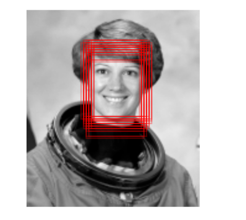
test_image = skimage.data.astronaut()
test_image = skimage.color.rgb2gray(test_image)
test_image = skimage.transform.rescale(test_image, 0.5)
test_image = test_image[:160, 40:180]

plt.imshow(test_image, cmap='gray')
plt.axis('off');

• 跑過一張圖片的所有cell來運算每個cell的特徵值

def sliding_window(img, patch_size=positive_patches[0].shape,
                   istep=2, jstep=2, scale=1.0):
    Ni, Nj = (int(scale * s) for s in patch_size)
    for i in range(0, img.shape[0] - Ni, istep):
        for j in range(0, img.shape[1] - Ni, jstep):
            patch = img[i:i + Ni, j:j + Nj]
            if scale != 1:
                patch = transform.resize(patch, patch_size)
            yield (i, j), patch
            
indices, patches = zip(*sliding_window(test_image))
patches_hog = np.array([feature.hog(patch) for patch in patches])
patches_hog.shape

• 可以發現在跑完整張圖片後，總計有33個檢測值，把這些檢測值在圖片上表示，可以看到下圖，他把訓練集合人臉資料一樣的特徵框起來

labels = model.predict(patches_hog)
labels.sum()

fig, ax = plt.subplots()
ax.imshow(test_image, cmap='gray')
ax.axis('off')

Ni, Nj = positive_patches[0].shape
indices = np.array(indices)

for i, j in indices[labels == 1]:
    ax.add_patch(plt.Rectangle((j, i), Nj, Ni, edgecolor='red',
                               alpha=0.3, lw=2, facecolor='none'))

Scikit-Learn在這邊講解的差不多了，這裡來整理一下：

1. Scikit-Learn介紹
2. 特徵工程(Feature Engineering)
3. 貝氏分類器(Naive Bayes Classification)
4. 線性迴歸(Linear-Regression)
5. 高斯函數(Gaussian Linear Regression)
6. 支持向量機(Support Vector Machines)
7. 決策樹(Decision Trees)
8. 隨機森林(Random Forests)
9. 主成分分析(Principal Component Analysis)
10. K-Means
11. 高斯混合模型(Gaussian Mixture Models,GMM)
12. 方向梯度直方圖(Histogram of Oriented Gradient, HOG)